MAY 4 2026: APP 2.0.0-beta44 has been released !
New improved internal memory controls should now work on all computers
May 1 2026: APP 2.0.0-beta43 has been released !
Improved internal memory controls (much more stable and faster on big datasets), fixed CPU image viewer, fixed Narrowband extraction demosaic algortihms.
Apr 29 2026 APP 2.0.0-beta42 has been released !
New improved Normalization engine, Fixed random crashes in integration, fixed RGB Combine & Calibrate Star Colors, fixed Narrowband extraction algorithms, new development platform with performance gains, bug fixes in the tools, etc...
Apr 14 2026: Google Pay, Apple Pay & WeChat Pay added as payment options
Update on the 2.0.0 release & the full manual
We are getting close to the 2.0.0 stable release and the full manual. The manual will soon become available on the website and also in PDF format. Both versions will be identical and once released, will start to follow the APP release cycle and thus will stay up-to-date to the latest APP version.
Once 2.0.0 is released, the price for APP will increase. Owner's license holders will not need to pay an upgrade fee to use 2.0.0, neither do Renter's license holders.
Hi all,
Several APP users indicated that APP was really slow with integration when they tried to integratie stacks of several 100s of frames. (APP versions up until and including 1.054)
In version 1.055 (soon to be released), I have improved integration speed significantly using 2 upgrades in the integration engine.
- First, reading from the file mapper on the harddisk, (containing all data/frames/layers of the integration) is now simultaneous with calculating the pixel stacks. This increases speed immediately with a factor of 1.5-1.75x depending on hardware configuration.
- Furthermore, because the integration is strongly limited by harddrive performance in the old integration engine, APP will now greatly reduce the amount of IO calls needed for integration by dynamically adjusting the Read and Write buffers for the file mapper. APP used to have fixed read/write buffers of only 8KiloBytes. Depending on the amount of system memory, these buffers can now become as large 1024 KiloByte or 1 MegaByte. If you integrate hundreds of frames, integration speed will be increased now with a factor of 2-10x on both SSD and conventional SATA/PATA drives from this improvement alone.
These two upgrades combined will give a speed increase with a factor of 2-20x largely depending on the hardware, which is a huge performance increase. The actual speed increase depends on lots of factors, like the amount and speed of CPU cores, the amount of memory available, harddisk latency and, the actual maximum read/write speeds of your harddisk.
Since numbers and graphs illustrate the differences better, I have been running lots of tests with different settings.
- First I presenst the results with the old integration module, before showing the results with the new integration module.
- To compare the speed with the old and new integration module I have integrated 100x 16MegaPixel RGB frames of a Nikon D5100 camera. In bytes this means data integration on 18GB worth of data. If Multi-Band Blending is used, this is 1.5x 18GB = 27 GB worth of data that needs to be integrated.
- Finally I will show the results of integrating 400 frames with the new integration module on both an SSD and a conventional harddrive.
I will show the final conclusions as well here, because it's a lot of information to consume and not everyone will be interested to see all the test results:
Final conclusions:
- the new integration module gives a very nice speed increase in integration, especially for APP users that integrate on conventional harddrives.
- the old integration module took 142 minutes to integrate 100 frames, and probably would have taken about 9-10 hours to integrate 400 frames.
- the new integration module can integrate 400 frames of 16Mega Pixels in 3 RGB channels on a conventional drive in only 27 minutes. This is a speed increase of 20x with only 4GB of RAM memory allocated to APP.
- more cpu cores will increase integration speed and
- more RAM memory allocated to APP will as well. Allthough the effect of more RAM memory wasn't tested, it's clear it will. With more RAM memory, APP can make the READ/WRITE IO buffers larger and that's one of the 2 improvements in the new integration module.
Clearly, this is a huge improvement. If you take the whole process into account from frame loading, calibration, star analysis, registration, normalization and integration. APP should now integrate stacks of several hundred frames within a couple of hours on a conventional drive.
Details of the test PC:
ASUS PRIME X399-A
AMD Ryzen Threadripper 1950X 16cores / 32 threads running at 3,8 GHz.
32GB DDR4 2400MHZ quad channel
Harddrives used in testing:
SSD : M2 Samsung SSD 960 EVO

Conventional drive : SATA-600 Western Digital WDC WD20EARS-00MVWB0

Graphics card is not shown since the GPU is not used yet in Astro Pixel Processor (but first testing with GPU enabled modules will start soon)
Operating System: Windows 10 professional


Details of testing:
Since this is very new hardware with lots of CPU cores and lots of memory, I will be running APP with only 4 cpu threads enabled and 4GB of memory in all tests, (except the last test to illustrate tinfluence of more CPU cores). This way, CPU power and Memory usage in the tests, will be much more comparable to the hardware specifications of the PC of the average APP user.
In all tests,
- Frame loading times reported, actually means loading the frames and applying registration parameters (so data interpolation with Lanczos-3) and applying normalization parameters.
- I use the reference composition mode to ensure that the field of view of the integration is exactly 16 Mega Pixels in 3 color channels. This equates to 184 MegaBytes of data per frame, since the integration is done in 32bits depth.
- and Lanczos-3 with no under-overshoot enabled
So 100 frames * 184 MegaBytes = 18GB of data. With MBB enabled this is 27GB of data that needs to be processed.
So 400 frames * 184 MegaBytes = 72GB of data. With MBB enabled this is 108GB of data that needs to be processed.
All graphs that are shown, show memory usage in time. You'll see separate regions in the graphs, first region is always frame loading, then LNC if enabled, then the actual integration, and the final peak is always analysis of the integration result for location, scale, noise and SNR.
All test duration times are reported in minutes for easy comparison.
Test 1: OLD integration module
Integrate 100 frames
no MBB
no LNC
average integration
no outlier rejection
using the SATA 600 conventional drive:
frame loading: 12 min
actual integration: 2min ! completely from cache !

using the M2 SSD drive:
frame loading: 12 min
actual integration: 2 min

Test 2: OLD integration module
Integrate 100 frames
no MBB
no LNC
average integration
outlier rejection: winsorized 2 iterations with kappa 3
using the SATA 600 conventional drive:
frame loading: 12 min
actual integration: 6 min ! integration completely from cache, no IO reads at all during integration !

using the M2 SSD drive:
frame loading: 12 min
actual integration: 6 min

Test 3: OLD integration module
Integrate 100 frames
MBB 10%
LNC 1x 4th degree
average integration
outlier rejection: winsorized 2 iterations with kappa 3
using the SATA 600 conventional drive:
frame loading: 13 min
LNC: 10 min
actual integration: 142 min = 2 hours 22 min ! REALLY SLOW !

using the M2 SSD drive:
frame loading: 13 min
LNC: 7 min
actual integration: 9 min

Summary of performance using the old integration module using these three tests:
- If the stack/integration size is less then the amount of system memory minus the amount of memory needed for the Operating System to do it's regular work, then integration will be done using memory caching if the Operating System's kernel supports this (most OS's will). This will give fast integration probably only limited by CPU power. This was the case for test 1 and 2 where integration on the SSD and the conventional harddrive were equally fast. This memory caching feature will only really be used if you have at least 16GB of memory in your system and will only benefit large stacks if you have much more memory installed. So for a stack of 100GB you would need to have 128GB of memory installed to have the integration done using OS memory caching.
- Test 3 wasn't performed using memory cache, in this case, the slow integration speed on the conventional harddrive reveals itself. Actual integration on the conventional drive took 142 minutes, or 2 hours and 22 minutes. On the SSD drive it took only 9 minutes. This slow integration was reported by several users.
- Frame loading is the same on the different harddrives. So IO on the harddisk doesn't have much influence here. In this case NEF frames were used, and NEF read speed is mainly limited by the NEF raw conversion itself.
- LNC is a process that happens between frame loading and the actual integration and it will benefit clearly from a faster harddrive.
The following test is a repeat of test 3, because that wasn't using the OS memory caching, now showing the behaviour of the new integration module with the 2 mentioned upgrades.
Test 3: NEW integration module
Integrate 100 frames
MBB 10%
LNC 1x 4th degree
average integration
outlier rejection: winsorized 2 iterations with kappa 3
using the SATA 600 conventional drive:
frame loading: 13 min
LNC: 9 min
actual integration: 7 minutes ! ( old integration module took 142 minutes) IO on the harddrive is used optimally now.

using the M2 SSD drive:
frame loading: 13 min
LNC: 6 min
actual integration: 6 min

First conclusions:
The new integration module managed to improve speed especially on the conventional drive
- speed improvement on conventional harddrive: form 142 minutes to only 7 minutes... That is a factor of 20x times faster !
- speed improvement on the SSD drive: from 9 minutes to 6 minutes... A modest speed increase for already fast integration.
The integration speed on the conventional and SSD drive are almost the same now, which must mean that integration speed now becomes much more limited to CPU power, which I'll demonstrate in test 5. Remember, in these tests I have used only 4 cpu threads and 4 GB of memory.
The next test is using the new integration module and we are now going to integrate 400 frames instead of 100 frames. We are going to check that 4 times as much frames will take 4 times longer to make sure that the application isn't slowing down for whatever reason. This will be a repeat of test 2, but with 400 frames.
Test 4: NEW integration module
Integrate 400 frames
no MBB
no LNC
average integration
outlier rejection: winsorized 2 iterations with kappa 3
using the SATA 600 conventional drive:
frame loading: 45 min
actual integration: 27 min
using the M2 SSD drive:
frame loading: 45 min
actual integration: 26 min

Conclusion: SSD and conventional drive have identical integration speed in this case with the new integration module. So it's clearly limited by other factors, on of them must be CPU power in this case. I showed only 1 graph, because they are more or less identical. Compared to test 2, we also see that frame loading and the actual integration scale linearly between integrating 100 frames or 400 frames. Frame loading duration increased from 12 minutes to 45 minutes, and integration duration increased from 6 to 26 minutes.
Test 5 is a repeat of test 4, but now with all 32 CPU threads enabled to check for dependence on CPU power, only shown for the SSD drive:
Test 5: NEW integration module with 32 CPU threads enabled in APP
Integrate 400 frames
no MBB
no LNC
average integration
outlier rejection: winsorized 2 iterations with kappa 3
using the M2 SSD drive:
frame loading: 43 min
actual integration: 9 min , compare to 26minutes using only 4 cpu threads

The additional left graph shows CPU usage, showing that all of the 32 cpu threads are used extensively by APP during integration.
Test 5 confirms, integration speed using the new integration module is now limited by CPU power.
Final conclusions:
- the new integration module gives a very nice speed increase in integration, especially for APP users that integrate on conventional harddrives.
- the old integration module took 142 minutes to integrate 100 frames, and probably would have taken about 9-10 hours to integrate 400 frames.
- the new integration module can integrate 400 frames of 16Mega Pixels in 3 RGB channels on a conventional drive in only 27 minutes. This is a speed increase of 20x with only 4GB of RAM memory allocated to APP.
- more cpu cores will increase integration speed and
- more RAM memory allocated to APP will as well. Allthough the effect of more RAM memory wasn't tested, it's clear it will. With more RAM memory, APP can make the READ/WRITE IO buffers larger and that's one of the 2 improvements in the new integration module.
Clearly, this is a huge improvement. If you take the whole process into account from frame loading, calibration, star analysis, registration, normalization and integration. APP should now integrate stacks of several hundred frames within a couple of hours on a conventional drive.
Additional information on integration: one of the main purposes of integrating our images is to reduce noise in the resulting integration and thereby increasing the Signal to Noise ratio.
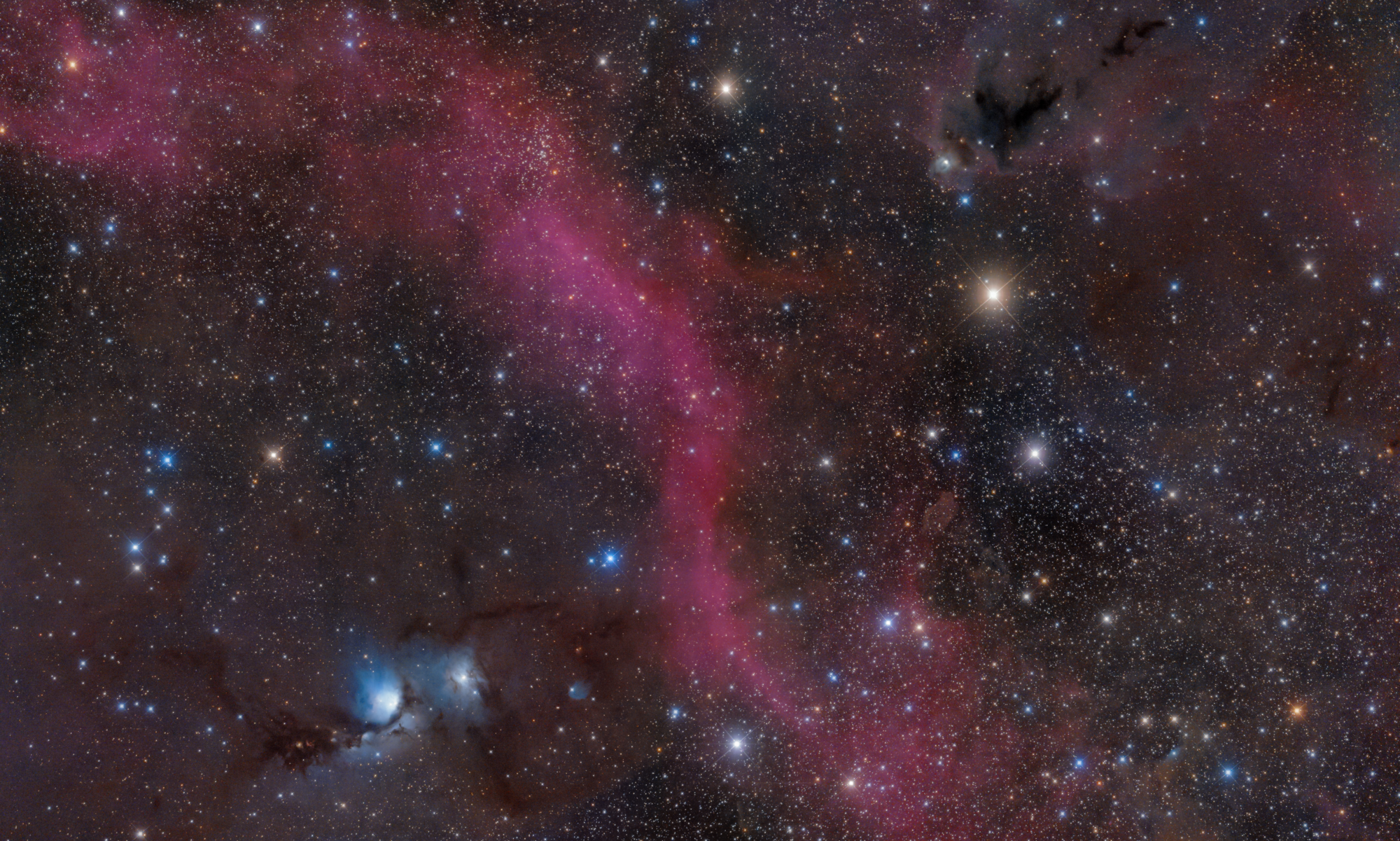
This particular dataset was made using a Nikon D5100 BCF mod with a 50mm Nikkor objective on a simple tripod. Single exposures were only 2,5 seconds on ISO 3200. Each image was shot with 2 seconds in between.
To illustrate how the noise droppes in integration i hereby show 3 images.
- single exposure of 2,5 seconds
- integration of 100 exposures giving total integration time of 250 seconds
- integration of 400 exposures giving total integration time of 1000 seconds.
To properly compare the frames, all 3 were corrected for gradients and background calibrated first. Then the single image and the 2 integrations were registered and normalized for location and scale/dispersion (multiple-scale) with each other and then saved. Shown are screenshots of APP showing a zoomed in part of the registered-normalized frames with the histogram visible. (The histogram that APP shows, is only of the data that is visible in the image viewer window, so in this case, the histogram shows the histogram of the zoomed-in data.).
The normalization ensures that we can properly compare the images using the exact same stretch parameters. Because I normalized for scale/dispersion, I basically normalized for noise. Noise is highly correlated to the dispersion of the data, because we only have stars and sky background. If there was clear nebulosity, the correlation with noise whould have been much lower. So the 3 images shown will show similar dispersion/noise and thus are visually compared for the amount of signal that is showing due to integrating more frames.
Single frame:

100 frame integration:

400 frame integration:

We can clearly see that 1 frame compared to 100 frames gives a dramatic increase in signal shown. 400 frames relative to 100 frames does show an increase but not as dramatic.
The maximal noise drop theoretically is the square root of the number of images used in the integration.
So 100 frames would give a maximal noise drop of 10. APP analyses each integration, the results can be found in the fits header:
SIMPLE = T / Java FITS: Thu Oct 12 14:40:46 CEST 2017
BITPIX = -32 / bits per data value
NAXIS = 3 / number of axes
NAXIS1 = 4928 / size of the n'th axis
NAXIS2 = 3264 / size of the n'th axis
NAXIS3 = 3 / size of the n'th axis
EXTEND = T / Extensions are permitted
BSCALE = 1.0 / scale factor
BZERO = 0.0 / no offset
DATE = '2017-10-12T13:04:00' / creation date of stack
SOFTWARE= 'Astro Pixel Processor by Aries Productions' / software
VERSION = '1.054 ' / Astro Pixel Processor version
STACK = 'stack ' / stack of lights
CFAIMAGE= 'no ' / Color Filter Array pattern
EXPTIME = 254.0 / exposure time (s)
LOK-1 = ' 1,76E-02' / lokation of channel 1
LOK-2 = ' 1,76E-02' / lokation of channel 2
LOK-3 = ' 1,78E-02' / lokation of channel 3
SCALE-1 = ' 8,62E-04' / dispersion of channel 1
SCALE-2 = ' 6,92E-04' / dispersion of channel 2
SCALE-3 = ' 8,21E-04' / dispersion of channel 3
NOISE-1 = ' 3,45E-04' / noise level of channel 1
NOISE-2 = ' 2,99E-04' / noise level of channel 2
NOISE-3 = ' 4,80E-04' / noise level of channel 3
SNR-1 = ' 2,70E+00' / Signal to Noise Ratio of channel 1
SNR-2 = ' 2,66E+00' / Signal to Noise Ratio of channel 2
SNR-3 = ' 2,13E+00' / Signal to Noise Ratio of channel 3
medNR-1 = ' 9,61E+00' / median noise reduction, channel 1
medNR-2 = ' 9,10E+00' / median noise reduction, channel 2
medNR-3 = ' 8,95E+00' / median noise reduction, channel 3
medENR-1= ' 1,95E+00' / effective median noise reduction, channel 1
medENR-2= ' 1,95E+00' / effective median noise reduction, channel 2
medENR-3= ' 2,47E+00' / effective median noise reduction, channel 3
refNR-1 = ' 9,67E+00' / reference noise reduction, channel 1
refNR-2 = ' 9,10E+00' / reference noise reduction, channel 2
refNR-3 = ' 8,92E+00' / reference noise reduction, channel 3
refENR-1= ' 1,97E+00' / effective reference noise reduction, channel 1
refENR-2= ' 1,95E+00' / effective reference noise reduction, channel 2
refENR-3= ' 2,48E+00' / effective reference noise reduction, channel 3
refNR-x : shows almost a noise drop for all channels of about 9, so that's nearly perfect.
400 frame would give a maximal noise drop of 20. Which is twice higer than the 100 frames:
SIMPLE = T / Java FITS: Fri Oct 13 14:08:33 CEST 2017
BITPIX = -32 / bits per data value
NAXIS = 3 / number of axes
NAXIS1 = 4928 / size of the n'th axis
NAXIS2 = 3264 / size of the n'th axis
NAXIS3 = 3 / size of the n'th axis
EXTEND = T / Extensions are permitted
BSCALE = 1.0 / scale factor
BZERO = 0.0 / no offset
DATE = '2017-10-13T19:02:48' / creation date of stack
SOFTWARE= 'Astro Pixel Processor by Aries Productions' / software
VERSION = '1.054 ' / Astro Pixel Processor version
STACK = 'stack ' / stack of lights
CFAIMAGE= 'no ' / Color Filter Array pattern
EXPTIME = 1014.0 / exposure time (s)
LOK-1 = ' 1,77E-02' / lokation of channel 1
LOK-2 = ' 1,77E-02' / lokation of channel 2
LOK-3 = ' 1,78E-02' / lokation of channel 3
SCALE-1 = ' 8,05E-04' / dispersion of channel 1
SCALE-2 = ' 6,77E-04' / dispersion of channel 2
SCALE-3 = ' 5,98E-04' / dispersion of channel 3
NOISE-1 = ' 1,88E-04' / noise level of channel 1
NOISE-2 = ' 1,68E-04' / noise level of channel 2
NOISE-3 = ' 2,64E-04' / noise level of channel 3
SNR-1 = ' 4,86E+00' / Signal to Noise Ratio of channel 1
SNR-2 = ' 4,58E+00' / Signal to Noise Ratio of channel 2
SNR-3 = ' 3,29E+00' / Signal to Noise Ratio of channel 3
medNR-1 = ' 1,78E+01' / median noise reduction, channel 1
medNR-2 = ' 1,64E+01' / median noise reduction, channel 2
medNR-3 = ' 1,64E+01' / median noise reduction, channel 3
medENR-1= ' 3,37E+00' / effective median noise reduction, channel 1
medENR-2= ' 3,43E+00' / effective median noise reduction, channel 2
medENR-3= ' 3,29E+00' / effective median noise reduction, channel 3
refNR-1 = ' 1,78E+01' / reference noise reduction, channel 1
refNR-2 = ' 1,64E+01' / reference noise reduction, channel 2
refNR-3 = ' 1,65E+01' / reference noise reduction, channel 3
refENR-1= ' 3,36E+00' / effective reference noise reduction, channel 1
refENR-2= ' 3,43E+00' / effective reference noise reduction, channel 2
refENR-3= ' 3,32E+00' / effective reference noise reduction, channel 3
refNR-x shows a noise drop of about 16-18, so almost reaching 20 😉
Finally. here are 2 JPGs of a single frame and the 400 frame integration:


Let me know if all of this is clear and if there are any questions.
Kind regards,
Mabula
Thanks !
