The HSL selective color works linearly and can be used on both linear and non-linear data.
In the tutorial, I show 4 different operations that you can perform on the data to selectively manipulate colors. Differences will be very subtle in most cases and it really helps if the computer monitor is well calibrated for the sRGB (or a wider gamut colorspace like Adobe 1998).
You need to select a color and the data range over which you want to correct this color. So you can only select blue pixels that are near the sky background level for instance.
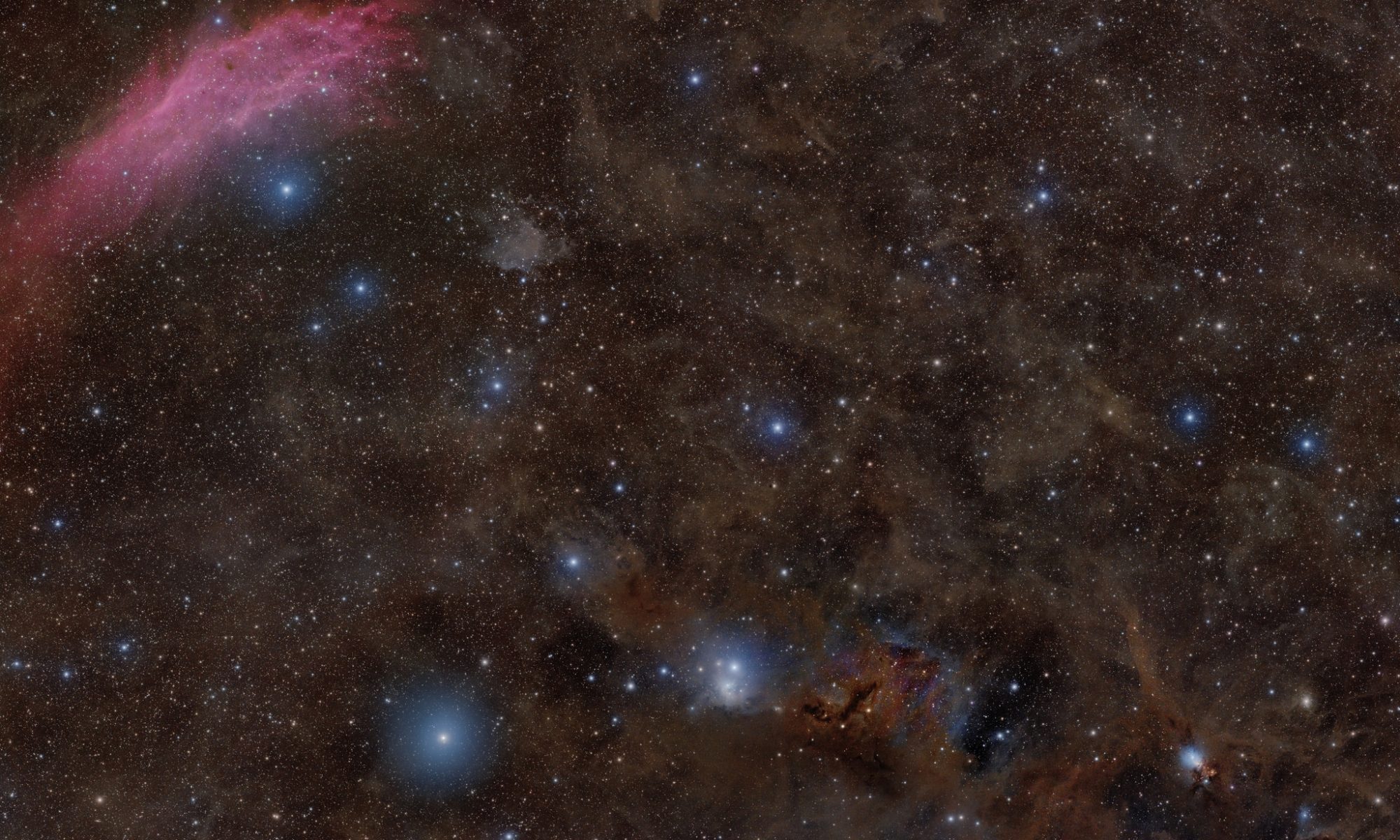
The sky background is at 0,0714 in the linear data in this particular image, as reported by the tool.
1) Reduce green pixels:
select green, 0%-100%
MA(GENTA) 1,00 ( pushing green to magenta, makes it white )
SAT -050,0 (reduce saturation in green pixels with 50%, makes them white)
calculate
apply
2) improve saturation in the blue nebula
select cyan 0,0% – 0,40% (so not saturating bright stars)
SAT +050,0 (increases saturation in cyan by 50%)
calculate
apply
select blue 0,0% – 0,40% (so not saturating bright stars)
SAT +050,0
calculate
apply
3) improve saturation in the red/magenta nebula
select red 0,0% – 0,40% (so not saturating bright stars)
SAT +050,0
calculate
apply
select magenta 0,0% – 0,40% (so not saturating bright stars)
SAT +050,0
calculate
apply
4) kill chromatic noise in the sky background
select ALL 0,0% – a little bit above the sky background value of 0,0714 = 0,080
SAT -100,0
calculate
apply
Finally to store this result:
CREATE and save to FITS
linear data is saved to the FITS file
click on cancel to stop the tool