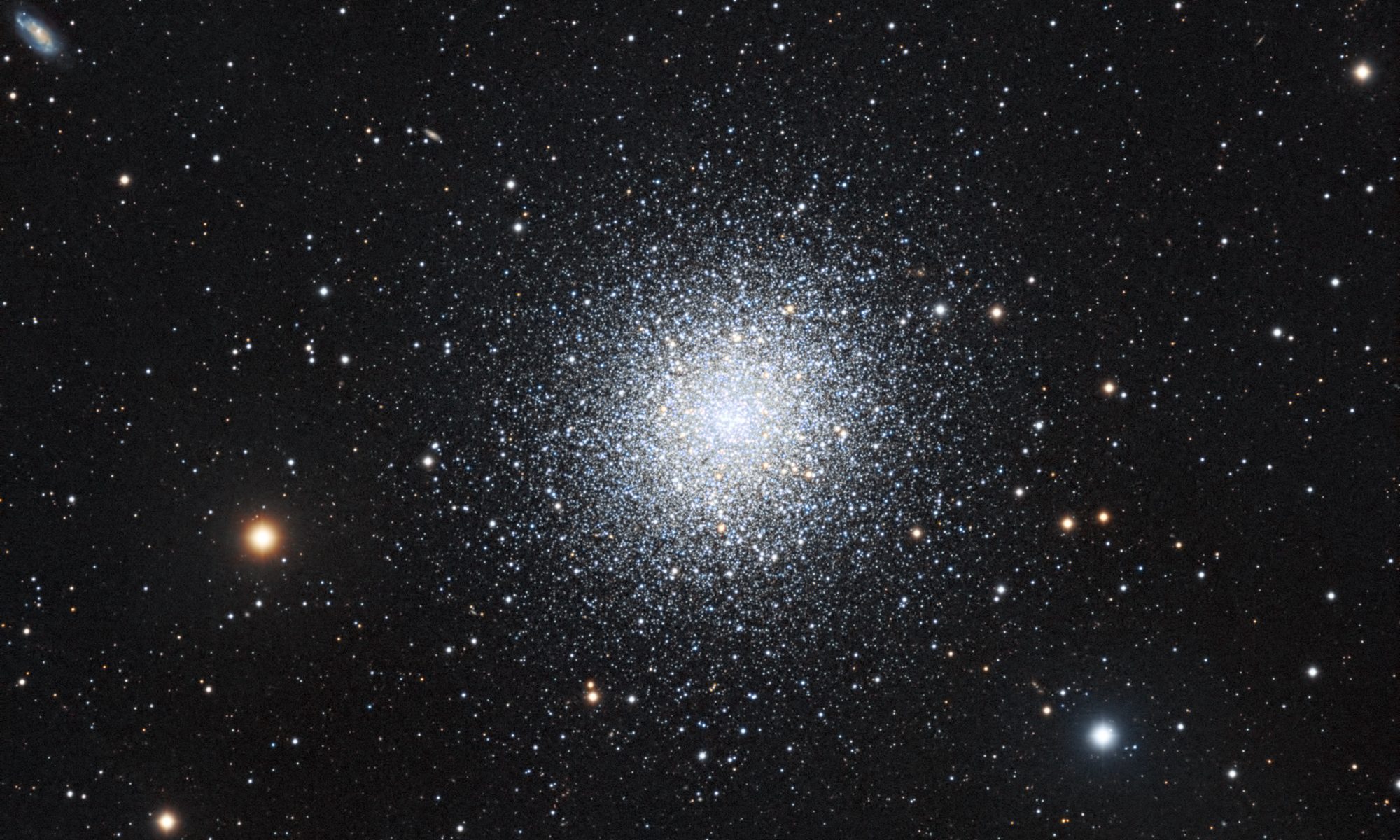
Data is courtesy of Stefan Lenz, Germany, and was captured in Namibia at the Kiripotib astrofarm.
Nikon D810a
Nikon VR 400mm F/2.8G
Sigma Art 135 F/1.8
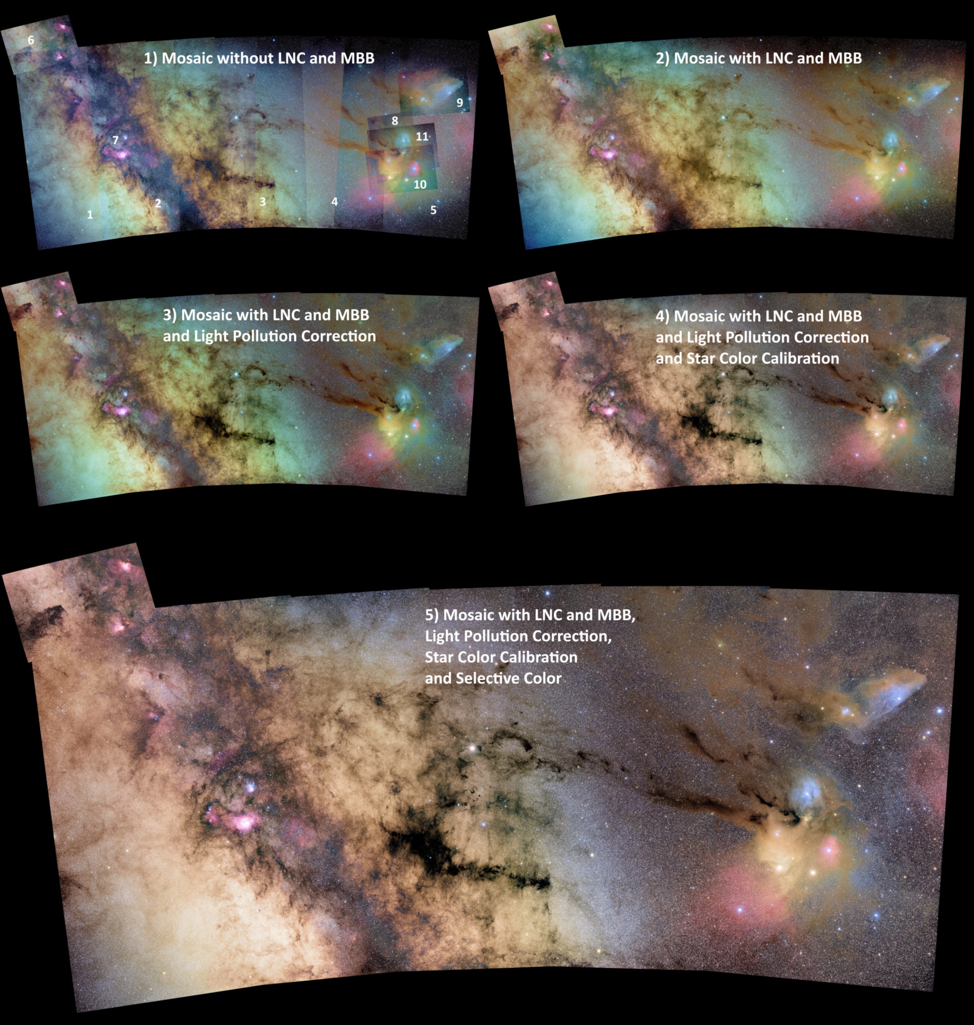
This is a very extensive tutorial consisting of several parts.
- Part 1: introduction
- Part 2: calibrate, register, normalize & integrate the individual mosaic panels
- Part 3: register, normalize, integrate the mosaic
- Part 4: perform gradient/light pollution correction and
background calibration to make a gray sky background - Part 5: star color calibration
- Part 6: HSL selective color
- Part 7: final stretching with the preview-filter
Part 1-3 deal mostly with how to create the mosaic from the individual exposures.

Part 4-7 are about post-processing the mosaic integration to a final image


Part 1: Introduction
The dataset is a multi-focal length mosaic, using 2 Nikon objectives of 400mm and 135mm focal length. The 400mm objective was used to captured more detail in interesting areas of the total Field Of View. Imaged is a widefield area that contains part of the Milkyway and the spectacular Rho Ophiuchi, Antares nebulosity complex.
Most data was shot with ISO 800, some frames were shot with ISO 400.
The different mosaic panels:
135mm:
Panel 1: 7x100s, 3x500s
Panel 2: 5x500s
Panel 3: 6x500s
Panel 4: 5x500s
Panel 5: 1x300s, 5x500s
All 135mm data was calibrated with a Bad Pixel Map and a MasterBias
400mm:
Panel 6 : 10x100s
5x300s
5x600s
Panel 7 : 10x300s
8x600s
Panel 8 : 4x600s
Panel 9 : 12x600s
Panel 10: 7x600s
Panel 11: 3x600s
All 400mm data was calibrated with a Bad Pixel Map, MasterBias, and a MasterFlat
Some remarks, tips:
- The most efficient and most robust way to register any data set as a mosaic is to first integrate the individual mosaic panels. Then register the mosaic using only the individual integrated panels.
- This holds for other mosaics as well. Don’t try to create a mosaic out of 100s of indivdual frames. First create the mosaic panels.
- To prevent integration/stack artefacts at the borders of the mosaic panels, use both Multi-Band Blending (MBB) & Local Normalization Correction (LNC) to reduce the amount of integration artefacts considerably.
- The actual Mosaic integration needs to be done, using MBB & LNC as well to correct illumination differences and to prevent the well-known mosaic seams.
- Regarding: Dynamic Optical Distortion Correction.In most cases, you can leave this disabled for the individual mosaic panel integrations. Only enable it if registration RMS is higher than 0.5 pixels and registration is visibly not correct. In the mosaic registration, you really need to have this enabled always.