Data is courtesy of Stefan Lenz, Germany, and was captured in Namibia at the Kiripotib astrofarm.
Nikon D810a
Nikon VR 400mm F/2.8G
Sigma Art 135 F/1.8
This is a very extensive tutorial consisting of several parts.
- Part 1: introduction
- Part 2: calibrate, register, normalize & integrate the individual mosaic panels
- Part 3: register, normalize, integrate the mosaic
- Part 4: perform gradient/light pollution correction and
background calibration to make a gray sky background - Part 5: star color calibration
- Part 6: HSL selective color
- Part 7: final stretching with the preview-filter
Part 1-3 deal mostly with how to create the mosaic from the individual exposures.

Part 4-7 are about post-processing the mosaic integration to a final image


Part 1: Introduction
The dataset is a multi-focal length mosaic, using 2 Nikon objectives of 400mm and 135mm focal length. The 400mm objective was used to captured more detail in interesting areas of the total Field Of View. Imaged is a widefield area that contains part of the Milkyway and the spectacular Rho Ophiuchi, Antares nebulosity complex.
Most data was shot with ISO 800, some frames were shot with ISO 400.
The different mosaic panels:
135mm:
Panel 1: 7x100s, 3x500s
Panel 2: 5x500s
Panel 3: 6x500s
Panel 4: 5x500s
Panel 5: 1x300s, 5x500s
All 135mm data was calibrated with a Bad Pixel Map and a MasterBias
400mm:
Panel 6 : 10x100s
5x300s
5x600s
Panel 7 : 10x300s
8x600s
Panel 8 : 4x600s
Panel 9 : 12x600s
Panel 10: 7x600s
Panel 11: 3x600s
All 400mm data was calibrated with a Bad Pixel Map, MasterBias, and a MasterFlat
Some remarks, tips:
- The most efficient and most robust way to register any data set as a mosaic is to first integrate the individual mosaic panels. Then register the mosaic using only the individual integrated panels.
- This holds for other mosaics as well. Don’t try to create a mosaic out of 100s of indivdual frames. First create the mosaic panels.
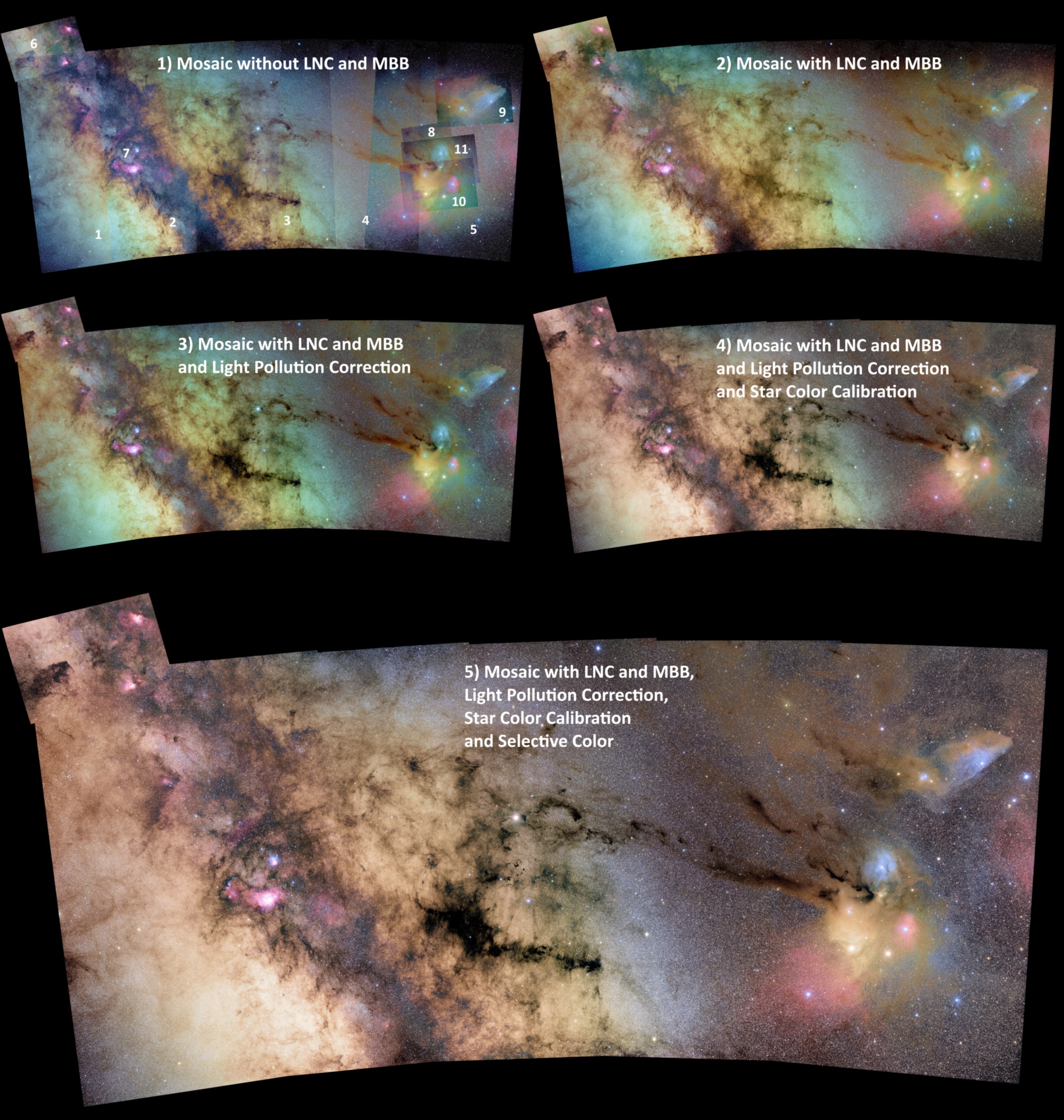
- To prevent integration/stack artefacts at the borders of the mosaic panels, use both Multi-Band Blending (MBB) & Local Normalization Correction (LNC) to reduce the amount of integration artefacts considerably.
- The actual Mosaic integration needs to be done, using MBB & LNC as well to correct illumination differences and to prevent the well-known mosaic seams.
- Regarding: Dynamic Optical Distortion Correction.In most cases, you can leave this disabled for the individual mosaic panel integrations. Only enable it if registration RMS is higher than 0.5 pixels and registration is visibly not correct. In the mosaic registration, you really need to have this enabled always.
Part 2: Calibrate, register, normalize & integrate the individual mosaic panels
Below, you can find the data processing settings that I used for the mosaic panels of both the 135 & 400mm data:
3) ANALYSE STARS
I have adjusted this a bit due to the very
high number of stars in Stefan’s images. This is due to
the excellent conditions in Namibia at time of exposure
and the long exposure lengths. The widefield data,
especially at 135mm is just full of stars
minimum star size = 10-20 (we favor the biggest stars
to use for analysis and registration, this really helps
when the data is full of stars like this…)
or enable the out of focus? FWHM > 12pixels setting to
reduce the star count, does help in this case
minimum stars 2000
maximum stars 4000
Remark:
For data with longer focal lengths and not so dense star fields.
The default settings in 3) are fine.
4) REGISTER
All default, only enabled Distortion Correction in case
of bad registration RMS (Bad is larger than 0.5 pixel).
So check the results after registration.
5) NORMALIZE
Defaults
6) INTEGRATE
Since we have less than 10 frames per panel, we
integrate with median integration.
weights: quality, since we have different exposure
lenghts, the images with higher star counts and better
SNR will have higher weights, slightly offset by
increased star FWHM sizes.
LNC: 1st degree 3 iterations
MBB: 5%
No Outlier rejection, unless needed due to artefacts.
The Bad Pixel Map of the Nikon D810a takes care
of all Bad/Hot Pixels in calibration.
Part 3: register, normalize & integrate the mosaic
Below, you can find the data processing settings that I used for the mosaic integration:
4) REGISTER
Set Panel 3 manually as reference. It’s the frame in the center of the Field of View.
Should prove a good starting point for the mosaic registration.
registration desciptors: pentagons
scale start 5
scale stop 10
enable dynamic distortion correction
disable same camera and optics
mode: mosaic
model: projective
Registration of mosaic was performed using 12000 starpairs with a precision of 0.41 pixels.
5) NORMALIZE
defaults, I used regular normalization to start with and that works fine in integration combined with further adjustments of LNC in this particular case. But you can always try advanced normalization, it should improve the initial normalization without LNC.
6) INTEGRATE
equal weights, average integration
LNC: 2nd degree 10 iterations
MBB 10%
No outlier rejection
Lanczos-3
scale 1.0x I kept the original image scale of the 135mm data since a 135mm frame was chosen as reference.
no Drizzle !
The final mosaic integration has dimension of 9245×18498 pixels.
Using the Batch Rotate/Resize tool, I rotated the result with 92 degrees counter clockwise.
Part 4: perform gradient/light pollution correction and
background calibration to make a gray sky background
Light Pollution correction & Background Calibration are both performed
with the Remove Light Pollution tool.
You need to place area select boxes on parts of the image where
there is no nebulosity or galaxy.
The area select boxes may contain a lot of stars, APP will disregard the
stars in the calculations, so the stars will not affect the outcome
of the correction model calculations.
Probably, the main key in getting a good correction, is to create the correction model, step by step, focusing on just part of the image.
Placing the area select boxes at the right place, takes some practice and experience.
The model flexibility can be adjusted, the model that looks correct with the lowest flexibility tends to be the best model, since it will be less vulnerable to
having placed some area select boxes at the wrong place.
Or:
The stiffness of the least flexible model allows for not placing the area
select boxes at exactly the right place.
Part 5: star color calibration
The Black Body & Extinction model is the default model
and is much more sophisticated than the Balance RGB model.
You will need to select areas with stars that are not strongly influenced by nebulosity.
The purpose is to select stars that represent main sequence stars. Realize that most of the stars in our images will be main sequence stars
that reside in our own galaxy, the Milky Way.
The model parameters, slope & constant, depend on the used camera
and the used filters, internally and/or externally
The constant parameters can be used to adjust for green/magenta cast.
If you need to lower/raise one of the constants lower/raise both constants a similar amount.
The Blue-Red slider needs to be used to perform the important white star calibration. Realize in this case, that most of the stars from the selected areas
will be red stars, since these live much longer than the blue stars. There are simply much more old red stars than young blue stars.
So most of the stars in your calibrated image, should normally be orange or red.
By adjusting the Blue-Red slider, you are informing APP the location
of white stars in the selected star population.
Adjust the slope values in such a way that the star populations in the
color-color diagrams nicely follow the model line.
Part 6: HSL selective color
The HSL selective color works linearly and can be used on both linear and non-linear data.
In the tutorial, I show 4 different operations that you can perform on the data to selectively manipulate colors. Differences will be very subtle in most cases and it really helps if the computer monitor is well calibrated for the sRGB (or a wider gamut colorspace like Adobe 1998).
You need to select a color and the data range over which you want to correct this color. So you can only select blue pixels that are near the sky background level for instance.
The sky background is at 0,0714 in the linear data in this particular image, as reported by the tool.
1) Reduce green pixels:
select green, 0%-100%
MA(GENTA) 1,00 ( pushing green to magenta, makes it white )
SAT -050,0 (reduce saturation in green pixels with 50%, makes them white)
calculate
apply
2) improve saturation in the blue nebula
select cyan 0,0% – 0,40% (so not saturating bright stars)
SAT +050,0 (increases saturation in cyan by 50%)
calculate
apply
select blue 0,0% – 0,40% (so not saturating bright stars)
SAT +050,0
calculate
apply
3) improve saturation in the red/magenta nebula
select red 0,0% – 0,40% (so not saturating bright stars)
SAT +050,0
calculate
apply
select magenta 0,0% – 0,40% (so not saturating bright stars)
SAT +050,0
calculate
apply
4) kill chromatic noise in the sky background
select ALL 0,0% – a little bit above the sky background value of 0,0714 = 0,080
SAT -100,0
calculate
apply
Finally to store this result:
CREATE and save to FITS
linear data is saved to the FITS file
click on cancel to stop the tool
Part 7: final stretching with the preview-filter
VIDEO soon to be released…
The preview filter settings in part 1 – 7 were:
DDP on, auto, saturation on
DDP preset 30%BG, 2 sigma, 0,0% base
The DDP preset affects the B(lack) and ST(retch) slider.
So set automatically by the DDP preset were:
B(lack): 0.05707
ST(retch): 0.07176
And then I manually set:
SAT: 0,30
SAT. TH : 0,0
CON:0,0
SHARP: 0,0
This is very strongly stretched with a lot of saturation
with the purpose of being able to easily see all problems in the data.
Makes correcting the problems much easier !
To make an image ready for publication,
we need to be less aggresive, to produce a more pleasing
final image.
B(lack):0.04600 The Black point needed to be a bit lower to prevent clipping on the black point which was noticable in the Pipe Nebula.
ST(retch): 0.0900 less aggresive, increase the ST slider to reduce the stretch
HL (HighLights): 5, to protect the highlights in the image from becoming too strongly stretched.
SAT(uration):35 this is a highy saturated result, in most cases, a value of 25-30 is fine.
SAT TH (Saturation Threshold):5 the higher the threshold, the higher the point in the datarange were saturation is actually applied. This will protect the sky background from injection chromatic noise by simply adding saturation on all pixels with all data values. Since I killed the chromatic noise in the sky background with the HSL Selective Color tool, we can set this value very low safely.
CON(trast):0.15 increased contrast to boost the nebula especially, regular values are 0,10 to 0,15